

A pivot band is calculated from prices that have already traded. A liquidation map describes positions that are still exposed. When the two line up, an abstract reference on the chart becomes something more concrete: a price interval containing identifiable financial risk.
That overlap appears in the TradeLean research. It is visible in the underlying position data, not merely in a bright screenshot. On Solana’s monthly resistance map, the 0.618–0.786 band held an average 20.98% of the relevant liquidation exposure, against 16.29% and 16.57% in the equally wide neighbouring bands. It led both neighbours in five of the six observed months. Ethereum’s weekly support and BNB’s quarterly resistance provide different, equally instructive examples.
The important question is how far that finding travels. Does the same band dominate on Bitcoin? Does a strong average survive a change of month? Are bright modelled clusters measuring the same thing as reported liquidation prices? And what happens when we stop choosing the attractive examples and display every test?
This study answers those questions with scheduled historical observations, fixed pivot geometry and explicit comparisons. It covers 6,728 complete position snapshots, 24 weekly dates and 334 instruments with usable comparisons. For the ten familiar cryptoassets examined in detail, all 80 combinations of timeframe and side are available below.
The finding
The overlap is real.
The conditions matter.
The 0.618–0.786 band coincides with elevated reported liquidation exposure in specific asset–timeframe–side combinations. The evidence supports a conditional relationship, not an invariant concentration across every asset or period. “Statistically significant everywhere” is not a result of this study.
How to read the comparisons
A positive comparison means that the target band contains a larger average share of reported exposure than either equally wide neighbouring band. A weaker or negative comparison means the band did not stand out in that particular test; it does not mean there was no exposure there. These exposure comparisons are distinct from statistical correlation, which is discussed separately in the cross-venue check.
Start with the six selected positive examples and the maps. The complete results and robustness checks remain available to show where the relationship holds and where it does not.
Start with the measurement
“Liquidity” describes more than one map.
A large resting limit order, a stop order and a leveraged position with a reported liquidation price can all be drawn as a horizontal band. Their economic meanings are different. The colour and shape of a chart cannot settle which one we are looking at.
Resting orders describe currently displayed willingness to trade. A liquidation price identifies a condition under which an exposed position may need to be reduced or closed. A stop is an instruction that becomes active after its trigger condition is met. A liquidation message records an event the venue has reported. The first is available depth; the second is potential forced flow; the third is conditional flow; the fourth is an observed message about an event.
| Layer | What it represents | What it does not establish |
|---|---|---|
| Order-book liquidity | Displayed bids and offers at a particular time and venue. | That the orders will remain available when price reaches them. |
| Reported liquidation exposure | Open notional associated with usable reported liquidation prices. | A guaranteed future amount of market buying or selling. |
| Modelled liquidation heatmap | A provider’s estimated distribution or intensity surface. | A complete, directly observed register of all accounts. |
| Captured liquidation messages | Events reported by an exchange’s liquidation stream or archive. | The entire stock of risk that existed before those events. |
The principal numerical result here concerns reported liquidation exposure: eligible open-position notional grouped by reported liquidation price. “Concentration” means the share located inside a defined price band. It does not mean immediately executable order-book depth.
This is also why the article does not add percentages from different maps. A modelled intensity of 30, a position share of 30% and $30 million of captured messages are not interchangeable quantities. Presenting them on one colour scale would create an apparent agreement that the measurements themselves do not justify.
Hyperliquid’s own documentation makes the mechanism relevant: liquidation eligibility depends on maintenance margin, and the mark price participates in the process. The response can include partial reduction rather than an instantaneous closing of all notional. A reported level is therefore a useful observation about risk, while its eventual execution remains conditional on account and market state. Hyperliquid’s liquidation mechanics ↗
Define the address first
The zone exists before the heatmap is inspected.
The test starts with a completed reference period. Let its high be H, its low L and its close C. The central pivot is P = (H + L + C) / 3, and the reference range is D = H − L. A ratio k becomes a price through P + kD above the pivot or P − kD below it.
The outer TradeLean band runs from 0.618 to 0.786 of D away from P. Its midpoint is 0.702 and its width is 0.168D. On resistance, the lower and upper boundaries are P + 0.618D and P + 0.786D. On support, the price interval runs from P − 0.786D to P − 0.618D. The ordering reverses below P; the width does not.
This geometry provides a fixed address for the observation. We do not first locate the brightest cluster and then move the pivot until the two coincide. Nor do we change the band width for an asset whose exposure happens to be spread more widely. The boundaries are determined by completed prices and the chosen reference period.
That independence is the useful connection between a pivot roadmap and a liquidity map. One establishes where to ask the question. The other supplies evidence about what is there. Neither needs to be treated as a mystical explanation for the other.
P + [0.618D, 0.786D]P − [0.786D, 0.618D]P = (H + L + C) / 30.168 × (H − L)The inner band, 0.146–0.236, is retained in the wider research and can be displayed in the interactive map. Its width is 0.090D. The familiar 0.184 reference is a label within that band, not its arithmetic midpoint, which is 0.191. This article’s principal comparison is the outer band; the two tests are not pooled.
The same formula can be applied to many instruments. That is a statement about the portability of a calculation. Whether risk concentrates at the resulting prices is a separate empirical question for each market, observation window and data source.
A bright band needs a fair comparison.
A broad interval will often collect more notional than a narrow one simply because it contains more prices. Comparing the outer zone with a single line would give the zone a built-in advantage. The primary test therefore compares three adjacent intervals of exactly the same width.
Moving outward from P, the near control is 0.450–0.618, the target is 0.618–0.786, and the far control is 0.786–0.954. Each spans 0.168D. They share the same exposure pool and the same observation timestamp. There is no opportunistic movement of a control toward a visibly empty region.
Under a uniform distribution across the chosen side of the pivot map, a band of width 0.168 would hold 16.8% of the pool. That number is a useful geometric reference. It is not a market-specific null model. Real exposure can be skewed toward current price, concentrated around a few accounts or distributed unevenly after a strong move.
The more demanding local question is whether the target beats both equal-width neighbours. BNB provides a useful example: its quarterly resistance target averages 16.81%, almost exactly the uniform reference, yet the two neighbouring intervals contain only 12.63% and 8.87%. A comparison with 16.8% alone would miss that local contrast.
We report the difference in percentage points and, where helpful, the relative uplift against the stronger neighbour. Those are different expressions. SOL’s 20.98% against 16.57% is approximately 4.40 percentage points of additional share, or 26.6% relative uplift. Calling the result “26.6 percentage points” would exaggerate it substantially.
Finally, winning this comparison does not make the target the largest possible interval on the chart. A different equal-width band closer to P could contain more exposure. Local superiority, global ranking and a causal explanation for the concentration are three different claims.
Interactive research workspace
Put the positions next to the roadmap.
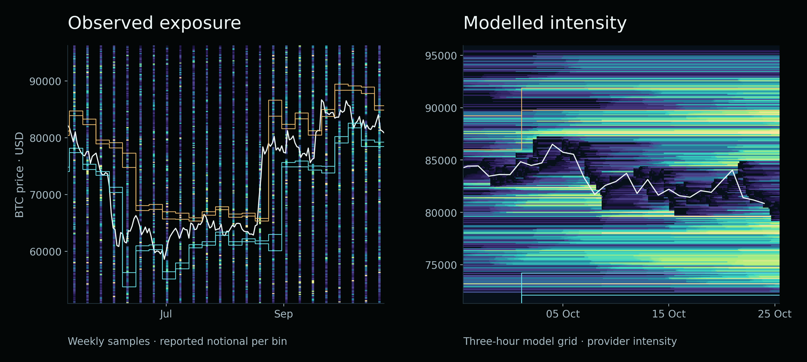
Start with observed exposure and switch between Bitcoin, Ethereum, Solana and BNB. The coloured columns are the actual weekly samples in the supplied research bundle. Blank time between columns is unobserved; it has not been filled by interpolation. The line traces daily closing prices from the same venue.
Observe the overlap.
Loading the archived research maps…
Nonlinear, within-map colour scale. Different assets do not share one dollar scale.
Use the pivot overlay to see whether a dense price bin sits inside, outside or across a band. Turn the inner bands off when they obscure the outer-zone question. Hover or tap a coloured cell to inspect its timestamp, price interval and notional. A price bin is a display unit; the exact zone percentages elsewhere in the article were calculated from the underlying position prices, not from the pixels.
The modelled view is deliberately a separate mode. It displays the archived CoinBoss model-2 grid for BTC, ETH or SOL, using the provider’s reported intensity units. It offers a denser visual surface, but it is not substituted for the directly observed position data. The model’s provenance and venue composition have not been independently verified for this study.
The colour-cap control changes display saturation, not the data. The observed maps default to a nonlinear scale capped at the 98.5th percentile of positive bin values so that moderate clusters remain visible beside very large ones. Values above that cap remain in every calculation. Raising or lowering the cap changes the image’s contrast, not the amount of risk in a zone.
Each asset uses its own map scale. A yellow cell on SOL and a yellow cell on BTC therefore do not necessarily represent the same dollar amount. For cross-asset comparisons, inspect the values or compare normalized shares in the results explorer rather than judging the brightness.
What the sample contains—and how a percentage is built.
The main dataset consists of historical Hyperliquid positions obtained through Vike. The sampling rule selects the first available Wednesday observation between 12:00 and 12:10 UTC. The broad study spans 24 scheduled dates, from 13 May through 21 October 2026. Available position pages were collected and checked for duplicates, invalid values and incomplete responses.
The combined catalogue contained 343 contracts. Usable comparisons were available for 334 instruments. Those are instrument identifiers, not 334 independent economic assets: additional markets and repeated underlying exposures appear in the catalogue. Of 6,728 complete snapshots, 6,680 contained nonzero eligible exposure for at least the relevant calculations. Applying multiple pivot bases, sides and zones produced 123,240 comparisons, not 123,240 independent experiments.
For a particular support-side observation, the denominator is the eligible notional with reported liquidation prices between P − D and P. The resistance-side denominator covers P through P + D. A price exactly at P is assigned to resistance only, avoiding a double count. The outer endpoints are included. Records with missing, nonpositive or unusable liquidation prices do not acquire an invented location on the chart.
The coordinate of a reported liquidation price q is k = |q − P| / D. The target numerator contains eligible notional at 0.618 ≤ k < 0.786 on the selected side. Divide that notional by the corresponding side’s pool and multiply by 100. The near and far controls use the same denominator. We first calculate a share for each snapshot and then average shares for the asset and combination being described.
This distinction prevents a large observation from silently redefining the question. An average share across snapshots asks about the typical sampled distribution. A ratio of all pooled dollars asks where the total sampled notional lies. Both can be informative, but they are not the same statistic. Repeated observations of a persistent position are also not new capital inflows and must not be added into a claimed cumulative accumulation.
For a broad cross-instrument summary, each eligible instrument’s average receives equal weight. A separate dollar-weighted summary would answer a different question and allow the largest markets to dominate. All public tables below retain the original definitions rather than changing weighting to improve the result.
Reference periods and the quarterly convention
Weekly pivots start on Monday UTC and use the completed previous week. Monthly pivots use the previous complete calendar month. Annual pivots use the previous calendar year. Only completed reference data enter an active grid.
The quarterly TradeLean convention in this dataset groups weekly bars by the quarter of their opening date. It is not automatically identical to calendar-day quarterly candles. The active transitions studied in 2026 occur on 6 April, 6 July and 5 October. This definition is preserved in every quarterly table and overlay; the calendar convention is not selected afterward to obtain a better fit.
Twenty-four weekly observations involve 24 weekly grids. The same observations on an annual basis involve one active annual grid. More snapshots do not create more independent annual periods.
Six examples show what “more exposure” actually means.
| Asset | Basis and side | Target | Stronger control | Gap | Relative uplift | Period wins |
|---|---|---|---|---|---|---|
| BTC | Weekly · support | 21.09% | 19.99% | +1.10 pp | +5.5% | 11 / 24 |
| ETH | Weekly · support | 24.50% | 19.56% | +4.93 pp | +25.2% | 11 / 24 |
| SOL | Monthly · resistance | 20.98% | 16.57% | +4.40 pp | +26.6% | 5 / 6 |
| BNB | Quarterly · TradeLean · resistance | 16.81% | 12.63% | +4.18 pp | +33.1% | 2 / 3 |
| AVAX | Monthly · resistance | 19.32% | 15.99% | +3.33 pp | +20.8% | 4 / 6 |
| LINK | Monthly · support | 26.83% | 20.62% | +6.21 pp | +30.1% | 3 / 6 |
These cases are selected to explain the findings, not to replace the full matrix. All compare mean shares inside their own asset, side and reference convention. A larger percentage for LINK does not establish a larger absolute liquidation pocket than BTC. Their pools can differ by orders of magnitude.
Bitcoin, weekly support: the target averages 21.09% against 19.99% in the stronger neighbour. The gap is approximately 1.10 percentage points, or 5.5% relative. This is a positive mean, but a fairly modest one. The target wins in 11 of the 24 weekly periods, so a slightly favourable average should not be described as dominance on most observations.
Ethereum, weekly support: the target averages 24.50%, compared with 19.56% and 17.77% in the controls. Its approximate 4.93-point lead over the stronger neighbour is a larger observed difference than Bitcoin’s. Yet its period count is also 11 wins out of 24. Magnitude and frequency tell different parts of the story.
Solana, monthly resistance: the mean target share is 20.98%, compared with 16.29% and 16.57%. Here the repeatability is the striking detail: five of six observed months beat both controls. It is the strongest monthly consistency among the prominently discussed examples, while still including one failure and partially observed endpoint months.
BNB, quarterly resistance: the target’s 16.81% compares with 12.63% and 8.87%. It wins in two of the three observed quarterly intervals. Only three intervals are represented, and they are not three complete independent quarters. This is an interesting quarterly contrast with a short period-level history.
AVAX and LINK: monthly resistance on AVAX averages 19.32% against a stronger control of 15.99%, with four of six monthly wins. Monthly support on LINK averages 26.83% against 20.62%, with three of six monthly wins. The latter has a larger average gap but a less consistent sequence. Ranking candidates by only one headline number would obscure that distinction.
The complete major-asset comparison
Change the asset. Keep the test unchanged.
The explorer exposes all ten assets, four pivot bases and two sides. Its three bars compare the mean target share with the two mean control shares. The matrix below is not filtered to positive examples: all 80 combinations remain selectable.
Follow the evidence.
Bars compare mean shares. “Above both” is descriptive, not a significance test. Period wins are shown separately.
Show the observed periods
Every combination
Select any cell. Teal indicates a positive mean gap; rose indicates a negative gap. Every cell also carries a signed number.
Open the printable full results matrix
There are 23 positive combinations out of 80 when “positive” means that the target’s mean share exceeds both neighbouring means. That is a descriptive count in this sample. It is not a 23-in-80 trading success rate, a reversal probability or a statistical significance statement.
Every one of the ten named assets has at least one positive combination in the matrix. This is a genuine cross-asset occurrence of the pattern, but it is weaker than a universal effect. Once eight combinations are available for each asset, choosing the best one afterward makes an attractive example easier to find. A claim intended to generalize must fix the combination or selection rule before examining new observations.
The matrix answers a useful practical question: where has the specific overlap appeared in the measured history? It also makes the contrary evidence immediate. Bitcoin’s familiar name does not make every BTC cell positive, and a favourable SOL monthly cell does not turn its other scales into the same result.
The complete derived CSV and per-period records are downloadable below. The explorer is a browser view of those tables, not a new live feed. Changing a control changes the selected published row; it does not rerun a hidden optimizer or query an exchange for current positions.
Read the historical maps at their actual sampling frequency.
A useful map shows where the reference bands stood as time passed. It must also show how often the underlying exposure was observed. The following four maps preserve the gaps between the Wednesday samples rather than making them look like a continuously monitored exchange heatmap.
Bitcoin’s weekly grid resets frequently. The displayed band can move because the previous week’s range changed even when a particular open position has barely changed. A cluster crossing into a new band after a reset is therefore different from new risk building at an unchanged level. The image is a way to locate those questions; it is not, by itself, a test of the mechanism behind the cluster.
Ethereum’s weekly support is numerically stronger than Bitcoin’s in the selected comparison. The chart adds the missing time context: the risk distribution and the pivot geometry both evolve. A few strong observations can contribute disproportionately to the mean. Looking along the full time axis is more informative than cropping around the brightest intersection.
Solana’s monthly map is less frequently reset, making it easier to compare observations within one active grid. The five-of-six monthly result should be read alongside both the changing band locations and the individual sampled distributions. It is a repeated local relationship in the observed window, not a promise that any price move into the band will reverse.
BNB illustrates the importance of the reference convention. Its quarterly overlay follows the TradeLean weekly-open grouping described above. A chart built from a different quarterly candle definition can shift the pivot and both boundaries. An apparent disagreement between two charts may be an input-definition difference rather than evidence that one of the maps is broken.
All four charts use the same venue for the daily prices and the position study. That removes one avoidable source of alignment error. It does not eliminate account-state uncertainty, missing liquidation-price records or the unobserved hours and days between samples.
A strong average and a repeatable effect are different findings.
An average can rise because of one unusually large episode. To ask whether the relationship recurs, we group the snapshots into their active pivot periods and compare the target with both controls again inside each period. For a monthly grid, the natural units are the observed months, not the individual positions inside a Wednesday snapshot.
SOL’s monthly resistance wins in five of six months. That is more informative than a single whole-window average because the advantage is not confined to one calendar interval. The losing month remains in the chart. May and October are only partially represented, and each month contains only a few scheduled observations. Five wins cannot be interpreted as a precise forecast probability.
AVAX’s four-of-six, LINK’s three-of-six and BNB’s two-of-three tell different repeatability stories. A research record should retain the mean gap, period count, length of coverage and frequency of wins. Combining them into a single “works” label discards exactly the information needed to judge whether the overlap deserves further monitoring.
Market regime is another potential confounder. A strong rally or decline changes where reported liquidation prices sit relative to earlier ranges. For this study, regime classification uses preceding daily information: a bullish observation requires a close above its 200-day simple moving average and an increase in that average compared with twenty days earlier. The bearish classification is the corresponding downside condition; other observations remain unclassified rather than being forced into a trend label.
The selected weekly-support ETH, quarterly-resistance BNB, monthly-resistance AVAX and monthly-support LINK combinations beat both controls in the separately pooled bullish and bearish observations. That extends their descriptive interest. It still does not demonstrate that every month, observation or future market regime will reproduce the same ordering.
There is an additional selection issue: regime tests of cases chosen for favourable full-sample averages are follow-up descriptions of those cases. They should not be presented as if the cases and the regime rule had been independently confirmed on a fresh dataset.
Ethereum’s daily history reveals what a headline average can hide.
A denser ETH series provides 168 usable daily observations from 8 May through 24 October 2026. One scheduled day lacked a snapshot in the specified window; another had no usable priced exposure. Those are exclusions, not zero-risk days. The series observes the same venue, so it adds temporal detail without becoming an independent exchange replication.
For quarterly support, the mean target share across this daily history is 22.67%, compared with 16.18% and 15.41% in the controls. That is a substantial positive descriptive contrast. Breaking it into active quarterly intervals changes how the result should be understood.
The observed second-quarter interval averages 33.56% in the target. The third-quarter interval averages 15.09%, and the October part of the fourth averages 24.77%. In the third interval, the far control holds 22.16%, beating the target. An assertion of unbroken quarterly-support dominance on ETH therefore fails the more detailed check.
Across individual daily observations, the target beats both controls on 78 of 168 days. The whole-window mean is positive even though a majority of days do not win. Large episodes can lift the average without creating a persistent daily condition. Both measurements are useful; they answer different questions.
This is why the article uses “observed concentration” rather than “always significant.” A large intermittent pocket may be important to the risk map. Describing it as a permanent feature would make the map less precise, not more confident.
What happens when the same test is applied across the market?
A collection of named examples is a starting point. A broader claim needs the same basis and side applied across all eligible instruments, without selecting a winner for each one. The broad summary first averages each instrument’s sampled shares and then gives those instrument averages equal weight.
| Basis | Eligible instruments | Target | Near | Far | Above both? |
|---|---|---|---|---|---|
| Monthly | 175 | 20.22% | 21.32% | 18.18% | No |
| Quarterly · TradeLean | 173 | 15.64% | 23.70% | 11.73% | No |
| Weekly | 176 | 24.40% | 16.84% | 30.11% | No |
| Annual | 130 | 6.17% | 12.85% | 5.00% | No |
For the combined support-and-resistance pool, the outer target does not beat both neighbours on any of the four bases. On the weekly basis it is ahead of the near control but behind the far control. On the monthly basis it is behind the near control. The quarterly and annual comparisons also fail to establish universal superiority.
This does not erase the positions measured inside SOL’s or ETH’s band. It changes the scope of the conclusion. Specific favourable combinations coexist with an unfavourable broader baseline. Both facts belong in the same article if the reader is to understand the result.
Support and resistance should also be retained separately. Pooling the two sides can hide a positive result on one side and a negative result on the other. Conversely, selecting the better side after inspection cannot be treated as proof that a side-independent effect exists.
The wider research also identifies candidates among less familiar contracts. Because those candidates emerge after a large search across instruments and settings, their immediate value is as a prospectively testable shortlist. Publishing only their successful cells would make the relationship appear more general than the measured evidence.
A different visual layer
Continuous heatmaps show a different kind of information.
The dense maps below are archived CoinBoss model-2 surfaces. The archive was saved on 25 October 2026; its grid contains 250 price centres and a sequence of three-hour timestamps. The plotted quantity is provider-reported intensity, not a directly observed sum of account notionals in our position sample.
These maps are valuable visual context. They make it easier to see the persistence and disappearance of modelled clusters and to compare their locations with the monthly pivot bands. They do not extend the 24 weekly position samples into a continuous account-level record.
The interactive map lets you switch between these two data types precisely so that the difference is visible. The observed mode labels bin values in dollars. The modelled mode labels them as intensity units. A cluster can be prominent in one and less prominent in the other because the providers are measuring or estimating different objects.
CoinGlass describes its liquidation heatmap levels as calculations based on market data and liquidation leverage levels. That is another reason to identify the provider and model rather than treating every heatmap as an interchangeable inventory. A well-designed chart should make the distinction easier to see. CoinGlass heatmap methodology reference ↗
Agreement between a model and a position-based observation is worth investigating. Calling it a second independent measurement of the same population would require more information about the model’s venue coverage, inputs, historical construction and dependence on the first source.
A precise overlay needs a common price basis.
A visual overlap is only as precise as the alignment of its two layers. Instrument, venue, price scale, timezone and reference-period convention all matter. BTCUSD on Bitstamp and a BTC perpetual elsewhere can have slightly different highs, lows and closes. Those differences move P and the zone boundaries.
The original TradeLean TradingView images are retained as chart context. Their instrument labels and attribution remain visible. They are not presented as newly downloaded position records or as numerical sources for the percentages reported in the results explorer.
The supplied CoinGlass image carries monthly pivot bands calculated from Bitstamp. Its price scale was calibrated from the image, and the approximate transition to the October grid is marked. The original timezone is not known. This is an illustrative cross-source overlay, useful for orientation but insufficient for extracting exact exposure shares from coloured pixels.
The historical position-map reconstructions take a different approach: daily prices and reported exposure come from Hyperliquid, and the overlay uses the stated completed reference data. This keeps the data basis consistent for the quantitative comparison. The reconstructed candles are labelled as reconstructions rather than being passed off as TradingView screenshots.
When two bands appear close, the first response should be to check their numerical boundaries, not to tighten the crop. A small price-basis difference can matter when a cluster lies near 0.618 or 0.786. Reporting the convention preserves the possibility of an independent reproduction.
Connect this study with the price roadmap.
The research builds on the geometric framework in the TradeLean pivot series. The walkthrough below explains the outer band as a price area. It does not claim to have measured the position sample used in this article. Keeping the two roles distinct makes it easier to see what the present study adds.
How to Find Market Tops and Bottoms With Pivot Points · YouTube ↗ · Playing loads YouTube media.
For the arithmetic behind the bands, start with Fibonacci pivot points: the map before the move. For how higher and lower reference periods interact, continue with Connecting annual, quarterly and monthly pivot maps. Different timeframes can point toward a similar price interval; that geometric confluence is still separate from measuring the exposure located there.
The additional evidence in this article is the measured distribution. Instead of stopping at “price reacted near a line,” we ask whether an independently defined price band contains more reported risk than appropriate alternatives at the observation time.
Binance and Bybit agree about some distributions. Is the agreement specific?
The extended study uses public Tardis archives to obtain a longer calendar view of captured liquidation messages. The usable main span covers 77 first days of months, from June 2020 through October 2026. There are 160 downloaded files, 153 nonempty files and more than 3.8 million source-message rows in the described extension.
After comparable price-history and contract filters, the extension provides comparisons for 1,390 exchange–contract markets and 812 symbols. Linear USDT contracts are retained; inverse contracts are excluded because their notional units require different treatment. One underlying traded on two venues is two market records, not two independent economic assets.
The first day of each month is a sparse, systematic selection. It is particularly sensitive to the moment of a monthly pivot reset. A multi-year calendar span therefore does not turn the archive into a representative sample of every trading day.
For the combined quarterly outer band, the reported Spearman correlation of contract-mean target shares between Binance and Bybit is approximately 0.881 across 449 matched markets. That is substantial descriptive agreement. But the near control is approximately 0.885 and the far control approximately 0.906. The target does not stand out as uniquely correlated.
The neighbouring intervals matter here for the same reason they matter in the main test. Two venues trade the same underlying market and experience related price movements. Shared low-activity intervals and zeros can also affect ranks. A high target correlation, considered alone, would overstate how specifically the 0.618–0.786 geometry explains the agreement.
This extension concerns captured messages, not the pre-event inventory of all potentially liquidatable positions. Bybit’s current stream documentation, for example, identifies its price field as a bankruptcy price. Multiplying that field by reported size should not quietly be renamed turnover at an actual market execution price. Bybit field definitions ↗ · Tardis archive documentation ↗
The cross-venue result is informative about agreement in the chosen message sample. It is not independent confirmation that a fixed ratio attracts liquidity on every asset.
A large position is part of the risk, not an inconvenience to remove.
If one account contributes most of the notional inside a band, the pocket is still there. Deleting that account to make the distribution look smoother would answer a different question. All position sizes remain in the primary calculations in this study.
Concentration among participants nevertheless matters for interpretation. A pocket spread across many accounts may persist differently from a pocket dominated by one account that can add collateral or close. The useful question is not whether a large position makes the original observation invalid. It is how dependent the pocket is on that position continuing to exist.
The sensitivity table in the supplied data removes the largest target position and recalculates the denominator. The selected positive cases are materially weakened by that exercise. For example, SOL monthly resistance’s target share falls to approximately 12.20% in that stress view, while its near and far controls are approximately 18.07% and 18.66%. This identifies participant concentration; it does not retroactively remove the original exposure.
A high percentage can also describe a very small pool. In a separate current stop-order observation, STX monthly support contained 100% of the eligible pool but represented one stop of roughly $2,100. An IMX inner-band example contained about 95.16% of its stop pool but only about $1,326.74 of target notional. Those are real observations with very different economic scale from a large derivatives exposure pocket.
A complete pocket card needs four values.
- Share: how much of the defined pool sits inside the band?
- Dollars: what is the absolute eligible notional?
- Participants: how many positions contribute to it?
- Largest contribution: how dependent is it on the biggest position?
For monitoring, add distance from current price and the age of the observation. A very large distant pocket, a small nearby one and a rapidly disappearing one are different conditions even if their normalized shares happen to match.
Concentration and accumulation are not the same process.
A snapshot tells us where eligible exposure sits at one time. Accumulation is a claim about how it arrived or changed. A zone’s share can rise while its dollar notional falls if the rest of the pool falls faster. Conversely, new notional can enter the band while its share drops because neighbouring exposure grows more quickly.
The preliminary approach test looks at neighbouring weekly observations exactly seven days apart, within an unchanged active pivot grid. Price must move outward from P toward the relevant band without having reached its near boundary. The same event definition is applied to each control relative to that control’s own near boundary.
Only instruments with at least three eligible events for every one of the three bands enter the comparison. On monthly resistance for core crypto contracts, the target averages 18.65%, against 17.03% and 16.50% in the controls: approximately 9.5% relative uplift over the stronger neighbour. Individually, 59 of 173 instruments beat both controls.
That is an exploratory conditional concentration result. The events for the three bands occur on different dates and are not matched for distance, volatility, movement speed or trend phase. Weekly observations also miss fast intraweek approaches. The test does not establish that the band itself caused positions to accumulate or that price was subsequently drawn into it.
A stronger accumulation test would observe absolute notional and composition at higher frequency before the approach, match distance and volatility, keep the active grid fixed and compare changes over identical windows. The causal story should wait for that design rather than being supplied by a vivid animation.
Turn a heatmap into a record you can actually review.
The best use of a liquidity roadmap is to make the observation precise enough to revisit. Start with the definition before the image: instrument, venue, reference period, timestamp and the two numerical boundaries. Save them. A later change in the band or the account population should not be confused with a change in price behaviour around an unchanged pocket.
Next identify the data layer. If it is a provider’s liquidation model, record the provider, model and display unit. If it is an observed-position map, record what makes a position eligible and what is excluded. If it is an order book, distinguish displayed depth from liquidity that might cancel. The same word “liquidity” is too imprecise for all three records.
Then quantify the pocket. Use the target’s dollar value, its share of a stated pool and the corresponding two control values. The share is useful for context, while dollars prevent a tiny pool from looking systemically large. Retain the number of positions and the largest contribution if those fields are available.
Finally, observe change without rewriting the starting point. Did target notional grow or shrink? Did its share change because the target changed or because the denominator changed? Did the biggest account remain? Did a new pivot period move the band through a previously stationary cluster? Those questions turn an appealing chart into a research record.
| Record | Why it belongs |
|---|---|
| Asset, venue and timestamp | Defines which market and state are being described. |
| P, D and band boundaries | Preserves the original geometry before the subsequent outcome. |
| Target, near and far values | Shows whether the pocket is distinctive locally. |
| Pool notional and target dollars | Separates proportional concentration from economic size. |
| Position count and largest share | Reveals dependence on a small number of accounts. |
| Next observation under the same definition | Allows change to be measured rather than narrated afterward. |
Price behaviour is a further observation. A cluster may be approached, bypassed, crossed rapidly or left untouched. Its existence does not specify a profitable entry, direction or exit. Evaluating a trading rule would require a precisely timed signal, execution assumptions, funding, fees, slippage and an independent assessment of outcomes.
The roadmap remains useful without making that additional promise. It tells the reader where measured risk is concentrated, which data support that description and whether the description survives the next observation.
What would justify a stronger conclusion?
There is a clear hierarchy. First establish that a pocket exists. Then compare it with fair alternatives. Then ask whether the comparison repeats across periods. After that, test a rule fixed before new data arrive. A claim that applies to all assets or all market conditions sits far beyond a few positive retrospective averages.
The dependence structure limits the present evidence. A position can remain open across weeks. Assets can move together. Pivot bases reuse overlapping price history. Treating every position, snapshot and timeframe as an independent trial would create artificial precision. The broad history has 24 dates, six observed months and only three active quarterly intervals.
There is also multiple testing. The major-asset block alone contains 80 combinations for the outer band. The wider research contains many more. The favourable cases in this article are selected for explanation after seeing the results. They cannot acquire a confirmatory p-value simply by being presented in a more polished chart.
An earlier conservative check of a limited family of period-level tests, using exact sign permutations and a Holm adjustment, did not obtain adjusted statistical significance. That does not make the observed percentages fictitious. It limits the claim that the short, dependent history has established a general rule beyond the selected sample.
The direct statement the evidence supports is therefore: the band contains measurable, locally elevated exposure in specific combinations, and some of those combinations show repeated period-level advantages. The next step is to freeze those candidates and rules, then observe data that were not involved in selecting them.
A prospective confirmation protocol
- Fix the asset, side, pivot convention and 0.618–0.786 boundaries before the new observation window.
- Retain the 0.450–0.618 and 0.786–0.954 controls unchanged.
- Fix the sampling schedule, eligibility rules and minimum coverage.
- Track target dollars, target share and the two control shares separately.
- Use period-level inference that acknowledges time and cross-asset dependence.
- Report all prespecified candidates, including failures, and account for the tested family.
- Reserve an untouched evaluation window or genuinely prospective observations.
A fresh reconstruction of the same history, a different palette or a second indexer of the same venue can help catch errors. None creates a new independent market sample.
A price zone becomes more informative when the risk inside it is measured.
The research finds an observable overlap between the outer TradeLean pivot band and reported liquidation exposure on several major cryptoassets. SOL monthly resistance combines a positive mean gap with five of six monthly wins. ETH weekly support has a larger mean concentration difference than BTC in the selected weekly comparison. BNB’s quarterly resistance illustrates why equal-width neighbours can be more informative than a uniform geometric benchmark.
Those findings are concrete enough to deserve continued investigation. They are also conditional enough that a universal statement would be inaccurate. The full matrix contains 23 positive and 57 nonpositive mean comparisons. The broad pooled summaries do not show dominance on every basis. The denser ETH history includes a losing quarterly interval. Cross-venue agreement is strong in the message archive but also strong in neighbouring controls.
The 0.618–0.786 band is a repeatable place to investigate risk. In the observed history, it coincides with elevated liquidation exposure in identifiable combinations of asset, side and timeframe. Whether that concentration is present now remains a question for the data.
That is the purpose of the liquidity roadmap: a defined address, a measurable state and a record that can be challenged by the next observation. The visual should bring those three things into focus.
Questions about liquidity heatmaps and pivot zones.
Does the study prove that every asset concentrates liquidity in the 0.702 zone?+
No. All ten major assets have at least one positive mean comparison among the eight combinations examined for each asset. However, only 23 of the 80 combinations are positive, the broad pooled summaries are not universally positive, and some positive averages have low observation-level repeatability. A claim covering every asset, timeframe and date is not supported.
Is a liquidation heatmap the same as an order-book heatmap?+
No. An order-book map displays resting bids and offers. A liquidation map concerns reported or estimated prices associated with leveraged-position liquidation risk. One describes displayed liquidity, the other potential forced-flow exposure. Their colours can look similar while representing different underlying quantities.
What does a positive number in the results matrix mean?+
It is the target’s mean exposure share minus the larger of the near and far mean control shares, in percentage points. It is not the mean of each snapshot’s minimum margin, which is a different operation. A positive number means local superiority of means in the selected sample; it is not a statistically significant p-value or a forecast return.
Why can the mean be positive when fewer than half the observations win?+
Magnitude and frequency differ. A few large concentration episodes can raise the average target share even when the target does not beat both controls on most dates. ETH’s denser quarterly-support sample illustrates this: the overall mean is positive, but only 78 of 168 daily observations win both comparisons.
Are the gaps in the observed heatmap missing liquidity?+
They are missing observations. The primary maps show scheduled weekly snapshots, with no temporal interpolation between them. A blank day does not imply there were no positions on that day. A black or low-intensity observed bin is different from an unobserved gap in time.
Does a brighter colour mean a larger dollar pocket across assets?+
Not automatically. Each map has its own nonlinear display scale, and the modelled view uses provider intensity rather than dollars. Compare the tooltip values or the normalized result tables. The display cap changes saturation only; all values remain in the underlying calculations.
Do large positions invalidate the result?+
No. Large positions are real exposure and remain in the primary sample. Their share tells us whether a pocket depends heavily on a small number of accounts. The largest-position-removal analysis is a sensitivity exercise about breadth, not a reason to erase the original risk.
Can these maps be treated as a live trading signal?+
These are archived research observations with stated sampling windows. They are not a live position feed or a tested trading strategy. A current risk assessment needs current data, while a strategy evaluation also needs explicit timing and execution rules, costs and independent outcome testing.
Inspect the numbers behind the visuals.
The public research files contain derived, anonymous tables and chart inputs. No API credentials, account identifiers or private account details are included. The interactive tools read these bundled files locally in your browser; they do not require an exchange login.
Sources, definitions and reproduction notes
- Main position data: supplied Vike / Hyperliquid historical research bundle, scheduled observations from 13 May to 21 October 2026.
- Daily price inputs: Hyperliquid, aligned to the venue used for the main position comparison.
- Modelled grids: archived CoinBoss model 2 for BTC, ETH and SOL, saved 25 October 2026; reported intensity units, not directly observed account notional.
- Supplementary historical messages: supplied Binance / Bybit archive analysis, first days of months from June 2020 to October 2026.
- Original chart context: TradeLean TradingView recordings and the supplied CoinGlass image. The CoinGlass–Bitstamp overlay is approximate and not a numerical source for the reported percentages.
- Primary documentation: Hyperliquid liquidation mechanics, CoinGlass heatmap definition, Bybit liquidation-stream fields, Tardis archive documentation and CoinBoss API documentation. Documentation checked 25 October 2026.
The 80 major-asset mean-share rows were recalculated against the bundled snapshot table. Exact zone percentages use positions’ reported liquidation prices. The binned maps are a visualization of derived exposure, so changing their number of rows or display cap does not redefine the target-band shares.
Boundary convention: the target includes 0.618 and excludes 0.786 in normalized coordinates. The resistance side owns the pivot price to avoid counting it twice. Largest-position stress views recalculate their denominator. Missing observations and missing liquidation prices are not replaced by zeros.
The study is descriptive research. It has not established a universal causal relationship, received independent peer review or evaluated trading performance. It reports measured comparisons and the limits of the supplied history.
Andrey
Founder of TradeLean. Engineer with a PhD, senior industry executive and long-time investor and trader. The work brings Lean thinking to chart analysis, historical research and market foresight.
About the author ↗Cite this research
Andrey. Liquidity Heatmaps & Pivot Zones: A Cross-Asset Study. TradeLean. 2026-10-25. https://tradelean.com/liquidity-pivot-zones
Join the conversation
Discussion
Questions, observations and thoughtful challenges to the research are welcome.
No comments published yet. Start the discussion below.
Leave a comment
Comments are reviewed before publication. Keep the discussion relevant and respectful; please avoid personal financial or account details.