

The most interesting part of an outer pivot zone is not the moment price touches its centre line. It is the sequence around the whole band: the approach, the time spent inside it, the attempts to leave and the position of the completed candle.
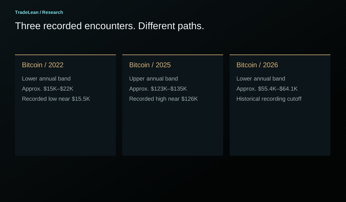
That is the focus of How to Find Market Tops and Bottoms With Pivot Points. In the recorded examples, Bitcoin's 2022 low, its 2025 high and its 2026 decline all intersect the outer 0.702 area of their respective annual grids. The S&P 500 example shows a market still trading within its upper band at the time of the October 2026 recording.
Those observations make the band worth examining. They do not make it an automatic reversal signal. This guide explains the calculation, the whole-zone rule and a practical way to distinguish a touch, a rejection and a breakout without letting the final outcome rewrite the original chart note.
How to Find Market Tops and Bottoms With Pivot Points
What is the 0.702 pivot zone?
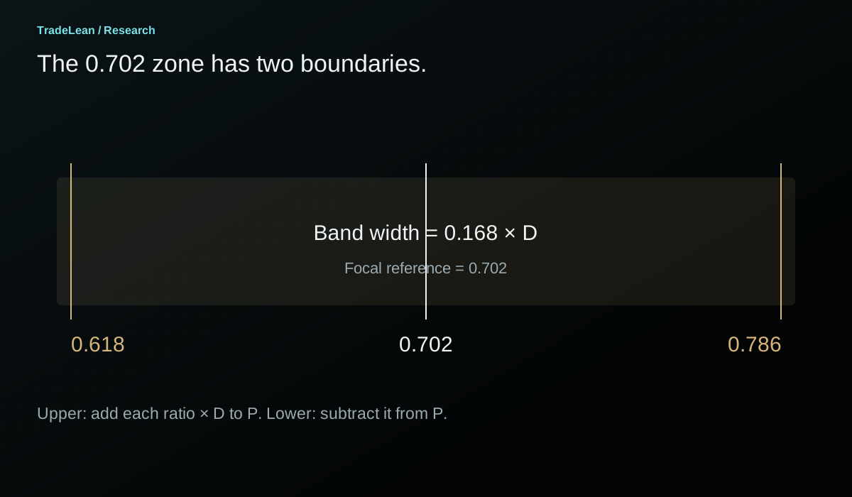
The TradeLean 0.702 zone is the band between the 0.618 and 0.786 multiples of the previous period's high-to-low range, placed above or below the central pivot. The 0.702 reference lies inside that band. It is a focal ratio, not a claim that all reactions happen at one exact price.
Let H, L and C be the high, low and close of the completed reference period. The central pivot is P = (H + L + C) / 3, and the range is D = H - L. The upper band runs from P + 0.618D to P + 0.786D. The lower band runs from P - 0.786D to P - 0.618D.
Writing the lower band in that order keeps its prices ascending. Subtracting the larger multiplier produces the lower price. It is a small arithmetic detail, but it prevents confusion when a chart label and a written range appear to be reversed.
The band width is 0.168D. Its width changes with the completed period's range, even though the ratios remain fixed. An annual band can therefore span thousands of dollars on Bitcoin while a monthly band on the same instrument is substantially narrower. The numerical size belongs to the inputs, not to a fixed percentage of the current market price.
| Component | Upper side | Lower side |
|---|---|---|
| Near boundary | P + 0.618D | P - 0.618D |
| Focal reference | P + 0.702D | P - 0.702D |
| Far boundary | P + 0.786D | P - 0.786D |
| Band width | 0.168D | 0.168D |
| Order when written as prices | Near boundary to far boundary | Far boundary to near boundary |
Calculation reference: TradingView: Pivot Points Standard
A worked example before looking at a market
Use a hypothetical completed period with H = 120, L = 80 and C = 100. The central pivot is 100 and D is 40. The 0.702 focal offset is 28.08, placing the upper focal line at 128.08 and its lower mirror at 71.92.
The band boundaries use different multipliers. At 0.618, the offset is 24.72. At 0.786, it is 31.44. The upper band therefore spans 124.72 to 131.44, while the lower band spans 68.56 to 75.28. Each is 6.72 price units wide.
Now consider three possible closing prices on the upper side. A close at 127 is above the near boundary but below the focal line. A close at 129 is above the focal line but still inside the band. A close at 132 is beyond the entire upper zone. Calling all three a breakout would erase information that the band was intended to preserve.
The mirror logic below P deserves the same care. A close at 70 is below the focal line but still inside the lower band. A close at 68 is beyond the far boundary. A close back at 76 has returned above the whole lower band. These are distinct locations even if each candle traded through the same focal level during the period.
Why a band is more useful than an isolated line
A perfectly thin line gives the eye an exact target. That can be useful for arithmetic and misleading for interpretation. Price can pass through a focal level, spend time near it, extend towards a boundary and then return without ever establishing a close outside the larger area.
The whole band provides a way to describe this uncertainty explicitly. A market inside the upper zone is still within the area being examined. It has not necessarily broken through resistance merely because its last traded price is above R 0.702. Equally, a move back below the focal line has not necessarily completed a rejection of the entire band.
A band also keeps several observations on the same map. The near boundary identifies the first encounter from the centre. The focal reference identifies a selected point within the area. The far boundary identifies the threshold for a move beyond the whole zone. Each serves a different descriptive purpose.
This does not mean that a wider band is always better. An area made arbitrarily broad can capture almost any turn and become impossible to falsify. The value here is that the boundaries follow a stated calculation. They are not widened after a low or high has already occurred.
The whole-zone rule
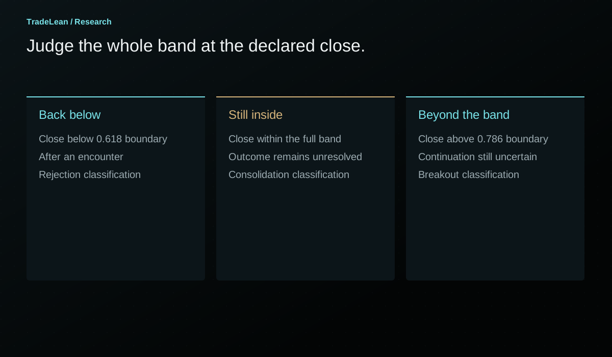
My rule in the walkthrough is to judge a breakout or rejection against the whole 0.618-0.786 band, using the chosen completed candle. For the annual examples, that observation is the monthly close.
On the upper side, a completed monthly close above the far boundary supports the description acceptance above the annual outer band. A completed monthly close below the near boundary, after price has tested the area, supports the description rejection back below the band. A close within the area leaves the market inside it.
On the lower side, reverse the direction. A close beneath the far lower boundary is beyond the whole support band. A close above the near lower boundary has recovered above the area. A close within it is still within it, even if the candle's wick briefly reached a dramatic low.
The encounter itself must also be defined. A period that never touched the band cannot be called a rejection from it just because it closed on the central side. A review needs an entry condition, a closing classification and an observation date. Without all three, attractive descriptions can replace reproducible events.
| Upper-zone closing position after a test | Description | Next question |
|---|---|---|
| Below P + 0.618D | Back below the whole band | Does the move continue towards an inner reference or revisit the zone? |
| Between P + 0.618D and P + 0.786D | Still inside the band | Is consolidation continuing, and where does the next completed close finish? |
| Above P + 0.786D | Beyond the whole band | Is that position retained or does a later close return inside? |
| Only an intraperiod print is beyond the boundary | Excursion beyond the band | What will the chosen candle close show? |
A reaction, a rejection and a reversal are different events
A reaction is an observed change after price encounters an area. It can be small, brief or quickly reversed. A rejection is a more specific description of price returning to the originating side of a defined band under a stated observation rule. A reversal is a broader claim about a change in the preceding move.
These terms should not be used interchangeably. A candle can react from the upper boundary and still finish within the band. A monthly candle can reject the band and still be followed by a later breakout. A larger cycle reversal can only be assessed with a longer record than a single touch supplies.
This is especially important when discussing a historical top or bottom. The completed chart makes the turning point obvious. At the first encounter, the eventual duration of the reaction was not yet known. Calling the initial touch a confirmed cycle top imports later information into an earlier observation.
A useful article can show the eventual outcome while preserving that timeline. State what was visible at the encounter, what became visible at the close and what was learned only later. The distinction makes the example more informative, not less compelling.
Bitcoin's 2022 lower-zone example
The recorded 2022 annual map has a pivot around $47,700, a lower inner reference near $40,000 and a lower outer band roughly between $15,000 and $22,000. These are rounded values from the walkthrough, intended to identify the areas shown on that chart.
Early in the year, the recording describes attempts beneath the lower inner area followed by a recovery towards the annual pivot. The sustained decline into the outer band occurs later. This matters because the outer-zone example is part of a sequence that includes an earlier recovery, rather than a straight line from the opening price to the eventual low.
By June, Bitcoin is trading in the lower part of the map. The final low described in the recording occurs in November near $15,500, close to the far side of the annual lower zone. The relevant monthly observation is that the selected chart does not retain a monthly close below the whole band during that example.
That combination is useful: the range was available from completed prior-period inputs, while the eventual low occurred much later. The map existed before the encounter. However, the fact that an area existed does not establish that a trade was entered there, that an exit was possible at an assumed price or that the same pattern wins across a representative sample.
The example should therefore be recorded as a historical fit to a defined annual zone. Its research value increases when it is compared with periods that behave differently, rather than when it is described as proof that all bear markets end at the same ratio.
Why the 2023 reset changes the interpretation
When the reference period changes, the grid changes. The 2023 annual map uses 2022's completed high, low and close. It is not the 2022 map moved forward with a new date.
The recording places the 2023 lower inner reference around $20,700 and discusses the recovery towards the new neutral range. This is a different observation from the prior year's reaction inside the lower outer band. One concerns the late stage of an old annual map; the other concerns location on a newly calculated map.
A review that merges them can create an artificial continuous signal. For example, the old outer support and the new inner reference might both help describe the recovery, but they do so with different inputs and different timestamps. Keep each grid's reference year attached to its labels.
The transition also explains why a market can be near an outer band in December and much nearer the centre of a new grid in January without a large price change between those dates. The mathematical frame has reset. That shift is not itself evidence of new buying or selling.
Bitcoin's 2025 upper-zone example
The 2025 map reverses the direction of the previous example. Its rounded pivot is near $80,000, its upper inner reference near $93,000 and its upper outer band approximately $123,000 to $135,000.
The walkthrough first identifies a completed move beyond the upper inner band in May. Later advances test the near side of the outer band. The October high is described around $126,000, which is within the broad numerical span of the area, although particular candle closes and feed details determine the precise location of each observation.
The important distinction is between trading inside the band and retaining a monthly close within it. The recording describes repeated tests without a retained monthly closing position through the area. Later weakness returns towards the annual pivot and eventually beneath the upper inner zone.
This is the mean-reversion example in the walkthrough: a move from an outer reference back towards the central part of the same map. It is not a promise that every outer-zone encounter returns to P. Some reactions are partial. Some revisit the band. Some break through it.
A careful review should also retain the time between the first test and the later decline. An observer who treated the first encounter as an immediate reversal could have faced a very different path from someone studying the final monthly rejection. The map identifies the area; the chosen event rule identifies the observation being evaluated.
Mean reversion: specify what is reverting to what
Mean reversion is often used loosely to mean any move against the preceding direction. Here the useful descriptive idea is a return from an outer pivot area towards an inner reference or the central pivot of the same grid.
The pivot is not an estimate of a statistical stationary mean. It is the arithmetic average of a previous period's high, low and close. A return towards it can therefore be described without claiming that price has a physical or economic obligation to return there.
A study should define its destination before reviewing outcomes. Returning from the upper outer band to R 0.184 is a different event from returning all the way to P. Counting either destination as success after seeing which one occurred would make the rule appear more flexible than it was originally specified.
Time also matters. A return within three completed candles and a return after a year of adverse movement are not equivalent. A period reset can make the destination ambiguous unless the study states whether the original grid remains the measuring frame after the reset.
For a practical record, write the originating zone, the defined event, the destination and the time window on the same line. That turns a compelling chart narrative into a question that can be examined across cases.
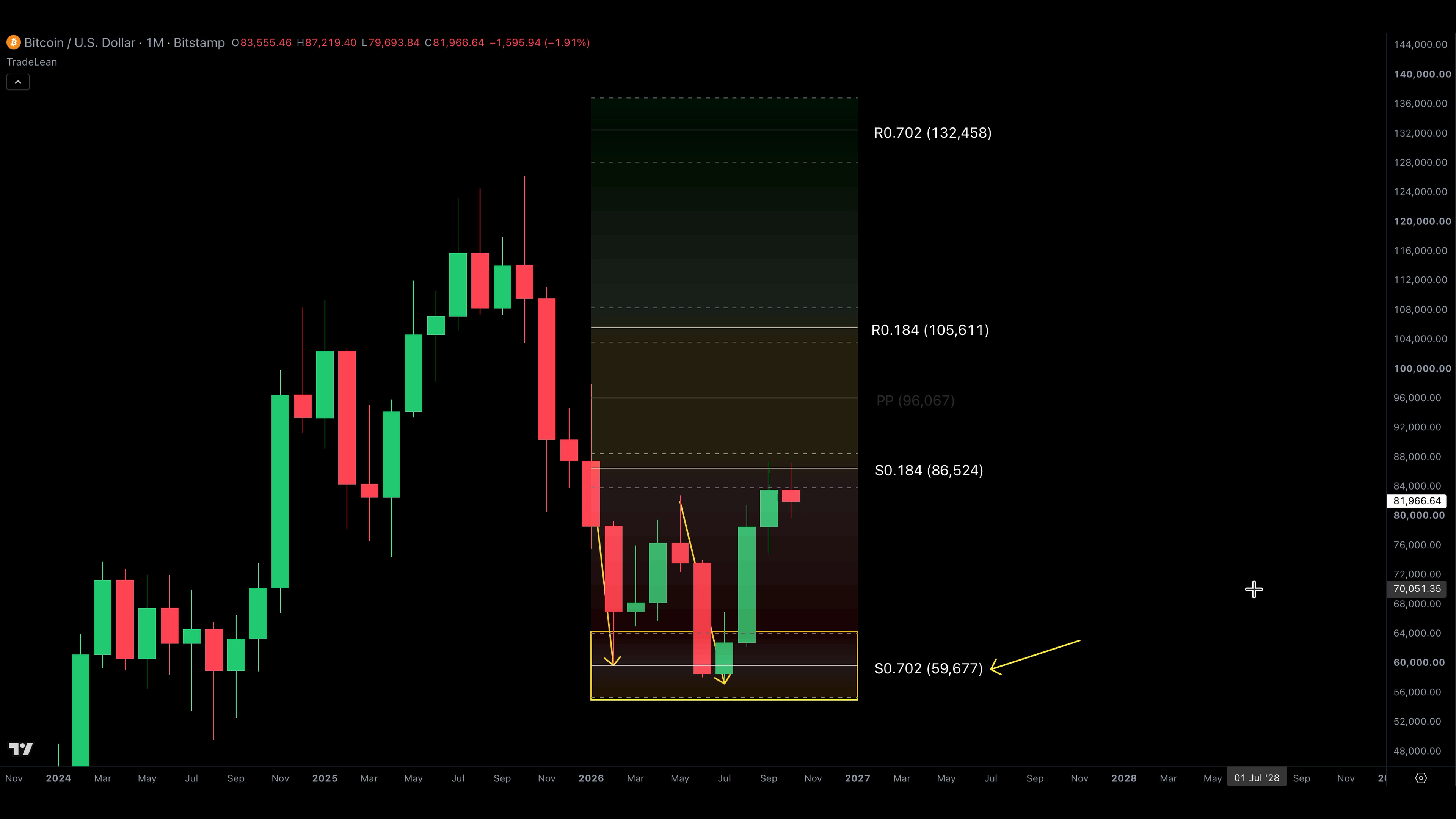
Bitcoin's recorded 2026 decline
In the October 2026 recording, the annual lower outer band is again relevant to the Bitcoin decline. The rounded reconstruction in the first article places its boundaries near $55,400 and $64,100, with S 0.702 near $59,700. The video describes a low around $58,000 during the observed period.
At that recording date, calling it the final low of an entire cycle would have gone beyond the available information. The useful statement is narrower: the observed decline reached the annual lower outer area and a subsequent recovery developed from that region in the recorded example.
The shape of the recovery still needs to be examined. How long did price remain in the area? Which monthly candles closed inside or outside it? How far did the recovery travel before encountering an inner annual reference? Those questions make better use of the map than treating the presence of a low inside a band as a completed argument.
The example is also a reminder that a lower grid can look weak while price is already at an annual outer reference. The multi-timeframe guide develops that conflict in detail. The outer zone is part of the context for evaluating a lower-timeframe breakdown, not an instruction to ignore every breakdown.
The S&P 500: remaining inside is an outcome
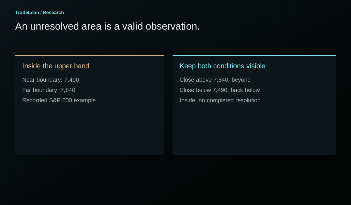
The recorded S&P 500 annual upper band runs approximately from 7,490 to 7,840. The walkthrough discusses a market that has reached that area after an advance and is still consolidating within it at the time of recording.
This is a valuable example precisely because the larger outcome was not yet resolved in the material. Under the whole-zone rule, a market still inside the band has not delivered either a retained breakout above it or a completed rejection below it. Waiting is a legitimate classification.
The recording identifies a monthly close above approximately 7,840 as the upper-side condition and a monthly close below approximately 7,490 as the lower-side condition. Those thresholds belong to that specific historical grid. They should not be presented as current signals on a page read months or years later.
The 0.382 reference near 7,000 and the inner band near 6,500-6,690 provide possible lower landmarks in the recorded scenario. Their presence does not imply that a decline to them was inevitable. A conditional map remains useful when it identifies what must first happen and where the interpretation changes.
What a failed outer zone looks like
An outer band can fail in several ways. Price may close beyond its far boundary and continue. It may consolidate inside the band for an extended period, making an immediate-reversal thesis unhelpful. It may reject the area briefly and then return through it. A review should identify which of these outcomes matters to the original hypothesis.
A failure of an immediate reaction is not necessarily a failure of a monthly-close rule, because those are different events. Conversely, a later eventual reversal does not rescue an earlier rule that required a reaction within a short window. The evaluation must use the original definition.
There is a temptation to add another condition after every difficult example. Require one more candle, switch to a smaller timeframe, use a different exchange, widen the band. Some refinements may be worth researching, but they should be treated as new hypotheses. Retrofitting them silently makes the original record impossible to assess.
A useful failure note contains the original condition, the first invalidating observation and the subsequent path. It is not a confession of error; it is part of the evidence needed to decide whether the method contributes anything beyond a visually attractive chart.
Build an event log rather than a highlight reel
Start with every eligible outer-zone encounter in the selected sample. Decide whether repeated visits within the same month count as one event or several. Decide whether a touch requires the candle's range to intersect the band or whether a close inside it is necessary.
Then classify the subsequent closing outcome. For example, record inside, returned to the central side or closed beyond the far boundary. Keep those categories mutually understandable. Do not count the same month as both a rejection and a breakout merely because its intraperiod high and low travelled widely.
Finally, measure what followed using a consistent horizon. The maximum favourable excursion, maximum adverse excursion and time to a defined destination often explain more than a simple win-or-lose label. If the result depends on a particular path through a daily candle, acknowledge that the daily data do not reveal the intraday sequence.
The denominator matters. Five striking reactions from five selected screenshots are not the same evidence as five reactions among fifty eligible encounters. An outer zone may be visually memorable even when many unremarkable encounters surround it.
| Event-log field | Example of a precise definition |
|---|---|
| Eligibility | First monthly candle whose range intersects the annual outer band |
| Reference grid | Annual, calculated from the previous completed year |
| Observation | Monthly close relative to both band boundaries |
| Destination | The originating side's 0.184 reference on the same grid |
| Horizon | A fixed number of completed monthly candles, stated before review |
| Failure | A specified opposite-side close or expiry without the destination |
| Data notes | Exchange, session, rounding and any missing observations |
A practical outer-zone review routine
First verify the inputs and calculate both band boundaries. Check the focal 0.702 line separately so a visual label cannot conceal an arithmetic error. Record the pivot period and the candle period used for acceptance.
Second, mark the first encounter and keep the chart visible up to that date only. Write the available scenarios before revealing later candles. Include continuation beyond the far edge and prolonged consolidation, not only a reversal towards the centre.
Third, advance the chart one chosen candle at a time. Record each completed closing position. If your interpretation changes, add a dated note rather than editing the old one. The record should show when a provisional idea became unsupported.
Fourth, review the result after the fixed horizon. Ask whether the band improved the description, whether the event rule was operational and whether the apparent success depended on information that was unavailable at the time. This is where the diagram becomes a research process.
You can use the fillable pivot-roadmap worksheet to keep the calculation and the later review together. Preserve the completed sheet even when the example is untidy. Those are often the cases that reveal which parts of the rule need clearer definitions.
Separate the first encounter from repeated tests
A zone can be visited several times during the same reference period. The first encounter after a sustained advance may differ from a fifth encounter after weeks of consolidation. Treating each touch as an unrelated observation can exaggerate the amount of evidence in a small sample.
Choose an event-counting rule. One approach is to count only the first eligible encounter per reference period. Another is to require price to leave the area by a declared distance before a new encounter can begin. Neither is universally correct; each defines a different research question.
Repeated tests also create a timing problem. If a market touches the band early in the month, leaves it and returns before the month closes, a monthly candle compresses those events into one range. An intraday reconstruction would contain more detail, but it would also require finer data and an explicit rule for separating visits.
Do not let the sampling resolution imply knowledge it does not contain. A monthly candle whose high and low cross both boundaries does not reveal the order of those crossings. A daily chart may narrow the uncertainty without fully removing it. The event log should preserve that limitation.
Distinguish a price-level study from a trading strategy
A study can ask whether outer-band encounters are followed by a return towards the centre. That is a legitimate price-behaviour question. It is not yet a trading strategy because it does not state when an order is placed, how it is executed or what limits a loss.
Turning the observation into a strategy requires additional definitions. A trigger based on a completed monthly close cannot be executed retrospectively at the intramonth high. A protective exit may be crossed during a gap. A target can be touched without a realistic assumption that every order was filled at that price.
Those details can materially change the result while leaving the chart illustration unchanged. The same diagram can therefore support an interesting research observation and an unattractive implementation. Keeping the two questions separate avoids attaching a performance claim to a chart that contains no execution record.
For the purposes of this article, the outer band is a reference area and the whole-zone rule is an observation convention. Any use in a trading process needs a separate assessment of risk, costs and suitability. The arithmetic alone cannot provide that assessment.
A comparison that would actually test the band
A fair comparison needs a baseline. If the hypothesis is that the 0.618-0.786 band identifies unusually important reactions, compare its eligible encounters with another declared rule using the same data and horizon. That might be a different fixed-distance band or a different ratio interval chosen before the evaluation.
The comparison should not give one method a favourable event definition and another an unfavourable one. If a touch qualifies for the TradeLean area, use a comparable touch definition for the baseline. If the evaluation waits for a monthly close, apply a corresponding closing convention throughout.
Also account for the fact that different bands are reached with different frequency. A more distant area may generate fewer observations and a different selection of market conditions. A high reaction rate in a tiny selected sample is not directly comparable with a lower rate across many routine encounters.
The useful output includes counts, uncertainty and the distribution of outcomes. A single average can conceal a small number of extreme reactions or many unresolved cases. The point of the exercise is to learn where the observation is useful and where it fails, not to force the preferred band to win.
The arithmetic of distance can improve the description
A band is defined in price units, but the distance from the current observation to that band can also be expressed relative to D. If a price is at P + 0.400D, the distance to the near upper outer boundary is 0.218D. This statement follows directly from the map and does not require a directional forecast.
That normalised distance helps compare different reference periods. Two markets can be a thousand dollars from an outer band and still be at very different relative locations if their completed ranges differ substantially. The same absolute distance is not the same position on the roadmap.
A distance measure should still be named accurately. It is distance relative to the chosen previous-period range. It is not an estimate of volatility, a probability of arrival or an expected return. Those would require additional definitions and data.
The measure is most useful as a descriptive field in the event log. It can help distinguish a reaction beginning immediately at a boundary from an interpretation made far away from the area and later justified by an eventual visit.
How to annotate an outer-band chart cleanly
Start with the two boundaries and the focal reference. Use a restrained fill for the area and retain enough contrast for the candles and axis labels. A chart with every ratio emphasised equally makes the outer band difficult to distinguish from the rest of the map.
Mark the observation date and identify whether the candle is complete. If the chart is a reconstruction from rounded spoken inputs, say so in the caption. If it is a still from the original recording, retain the platform attribution and the visible instrument labels.
Add only the later observations needed to explain the case. A first encounter, a chosen close and a later destination usually convey more than arrows on every candle. The annotations should help a reader reconstruct the sequence without implying that every movement was anticipated.
Finally, show the failure condition near the interpretation. A chart that displays a beautifully shaded support area but no possible invalidation encourages the reader to treat the region as a guarantee. A clear alternative path keeps the visual aligned with the conditional nature of the analysis.
Questions about the outer band
Is 0.702 the exact midpoint of the zone?
Yes, for the outer band the arithmetic midpoint of 0.618 and 0.786 is 0.702. That symmetry is specific to these boundaries. It does not imply a probability distribution centred on the focal line, and it does not make the focal line an execution instruction.
Why not use the standard 0.618 line alone?
The standard Fibonacci pivot calculation includes a 0.618 reference. The TradeLean presentation adds a defined surrounding area and emphasises its 0.702 focal reference. The choice changes how the chart is read, while the underlying pivot and high-to-low range remain the same. Whether that presentation improves a specific decision process is a separate research question.
Does a wick outside the zone invalidate it?
That depends on the rule being evaluated. In the annual examples discussed here, the monthly close is the stated observation. An intramonth excursion is therefore recorded but does not satisfy a monthly closing condition. A strategy with an intraday invalidation rule would be a different strategy and could experience a different outcome.
Can a support zone become resistance?
Price can approach the same calculated area from the opposite side after moving through it. The geometry does not change merely because the direction of approach changes. Record the new approach and the relevant closing condition rather than assuming that the previous descriptive label determines the next reaction.
Does every large move end at an outer zone?
No. The grid permits moves beyond the 0.702 band, including towards 1.000 and higher multipliers. Some large moves turn elsewhere. The selected examples explain why the band is a focus of the TradeLean approach; they do not establish a universal law or a guaranteed top-and-bottom detector.
What should be read next?
The price-location guide explains the journey from the centre towards an outer band. The multi-timeframe guide explains why an outer area on one grid can overlap an inner or central reference on another. Together they provide a more complete context than an isolated zone touch.
Check the calculation.
Enter completed-period prices to verify the focal levels and band boundaries. These inputs are illustrative and do not request live market data.
Your pivot grid.
| Reference | Lower side | Upper side |
|---|---|---|
| 0.184 line | 86,472.27 | 105,461.07 |
| 0.702 line | 59,743.47 | 132,189.87 |
Using the rounded Bitcoin example.
Andrey
Founder of TradeLean. Engineer with a PhD, senior industry executive and long-time investor and trader. The work brings Lean thinking to chart analysis, historical research and market foresight.
About the author ↗Join the conversation
Discussion
Questions, observations and thoughtful challenges to the research are welcome.
No comments published yet. Start the discussion below.
Leave a comment
Comments are reviewed before publication. Keep the discussion relevant and respectful; please avoid personal financial or account details.
Educational research, not personal investment advice. Historical examples and hypothetical illustrations do not establish future performance. Risk Disclaimer.